by Suraj Rampure (suraj.rampure@berkeley.edu)

Often, we read that logistic regression models the log-odds of an event. What exactly does that mean? Where does the sigmoid function come from?

First, some context. Typically, we study binary classification – that is, classifying a test point $x$ as belonging to class 1 or class 0 (for example, determining whether or not a certain patient has breast cancer, where $x$ is all of their health information).

In order to do this, we model the probability of a point belonging to either class, and use some cutoff/threshold value to determine when we predict class 1 vs. class 0. We use logistic regression to do this – logistic regression is a form of regression that takes in a set of variables and outputs a probability, that is, a continuous value between 0 or 1. To be clear, logistic regression on its own is not a form of classification. In order to use logistic regression for classification, we require a decision boundary.

As a concrete example, suppose we somehow predict that the probability that one certain individual has breast cancer to be 68%. If we choose a decision boundary of 50%, that would mean any individual with a probability greater than (or equal to) 50% we would predict to have breast cancer, and any individual with less than 50% we would predict does not have breast cancer. In this case, with a 50% decision boundary, we would say this individual does have breast cancer, but with a 70% decision boundary, we would say they do not.

Moving forward, $p$ will refer to the probability of a point belonging to class 1 (hence, $1-p$ is the probability it belongs to class 0).

In statistics, we say that the "odds" of an event that occurs with probability $p$ is $\frac{p}{1-p}$. Sometimes this is referred to as "odds-in-favor", as opposed to "odds-against" (or $\frac{1-p}{p}$, as is commonly used in sports betting). The odds of an event with $p = \frac{2}{3}$ is 2, sometimes denoted as $2:1$ or "two-to-one".

By log-odds, we quite literally mean $\log(\frac{p}{1-p})$ (with $\log$ representing the natural log, $\ln(\cdot)$). Suppose we set the log-odds of $p$ to some value $\alpha$, e.g. $\log(\frac{p}{1-p}) = \alpha$. We can actually solve for $p$ in this expression:

$$\begin{align*}\log(\frac{p}{1-p}) &= \alpha \\ e^{\log(\frac{p}{1-p})} &= e^{\alpha} \\ \frac{p}{1-p} &= e^{\alpha} \\ p &= e^{\alpha} - pe^{\alpha} \\ p(1 + e^{\alpha}) &= e^{\alpha} \\ p &= \frac{e^{\alpha}}{1 + e^{\alpha}} \\ &= \frac{e^{\alpha}}{1 + e^{\alpha}} \cdot \frac{e^{-\alpha}}{e^{-\alpha}} \\ \implies p &= \frac{1}{1 + e^{-\alpha}} \end{align*}$$

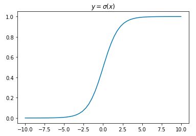
This resulting function $\alpha \mapsto \frac{1}{1 + e^{-\alpha}}$ is referred to as the sigmoid function, $\sigma(x) = \frac{1}{1 + e^{-x}}$.

Looking at a graph of $\sigma(x)$, we see that it accepts any value in $\mathbb{R}$ as an input, and outputs values in the range $[0, 1]$ – perfect for a probability distribution.

Now, recall, we set the log-odds of $p$ equal to $\alpha$. Instead, we can set the log-odds equal to some linear function of $x$, and optimize this function.

$$p = \frac{1}{1 + e^{-(\theta_0 + \theta_1x)}}$$

And, since $p$ represents the probability of our test point $x$ belonging to class 1, we can be more specific and say

$$P(Y = 1 | x) = \sigma(\theta_0 + \theta_1x) = \frac{1}{1 + e^{-(\theta_0 + \theta_1x)}}$$

where $Y$ is the class of point $x$.

We also don't need to restrict ourselves to using a single scalar input variable. In vector form, if we say $\theta = \begin{bmatrix} \theta_0 & \theta_1 & ... & \theta_k \end{bmatrix}^T$ is our weight vector and $\phi(\textbf{x})$ is our feature vector, i.e. $\phi(\textbf{x})= \begin{bmatrix} 1 & \phi_1(\textbf{x}) & \phi_2(\textbf{x}) & ... \phi_k(\textbf{x}) \end{bmatrix}^T$, we can say

$$\boxed{\begin{align*} P(Y = 1 | \textbf{x}) = \sigma(\phi^T(\textbf{x})\theta) &= \frac{1}{1 + e^{-\phi^T(\textbf{x})\theta}} \\ &= \frac{1}{1 + e^{-(\theta_0 + \theta_1\phi_1(\textbf{x}) + ... + \theta_k\phi_k(\textbf{x}))}} \end{align*}}$$

(Notice, we use $\textbf{x}$ to represent a vector, and $x$ to represent a scalar.)

As a concrete example, suppose we want to determine the probability of a baby growing to be over 6 feet tall, given their mother's height $x_1$, father's height $x_2$, and height at age 2 $x_3$. We can say $\textbf{x} = \begin{bmatrix} 1 \\ x_1 \\ x_2 \\ x_3 \end{bmatrix}$. Suppose we let one feature be a bias term, another feature be the average of their parents' heights and a third be the $\sin$ of their age 2 height; we could then say $\phi^T(x) = \begin{bmatrix} 1 & \frac{x_1 + x_2}{2} & \sin(x_3) \end{bmatrix}$ (these aren't necessary good features, as this is just an example). Since this is a linear model, of course, we'd have $\theta = \begin{bmatrix} \theta_0 \\ \theta_1 \\ \theta_2 \end{bmatrix}$. Then,

$$P(Y = 1 | \textbf{x}) = \sigma(\phi^T(\textbf{x})\theta) = \frac{1}{1 + e^{-(\theta_0 + \theta_1\frac{x_1 + x_2}{2} + \theta_2 \sin(x_3))}}$$

Then, using the appropriate loss function and a training set, we could determine the optimal set of weights $\theta$ to create the best predictor. We've now performed logistic regression, but we haven't yet built a classifier – a classifier outputs "1" or "0", and we have a function $P(Y = 1 | \textbf{x})$ that outputs continuous values in the range $[0, 1]$.

Suppose the cutoff boundary for our classifier is $p_0$, meaning probabilities greater than or equal to $p_0$ are classified as 1, and below $p_0$ as 0. Then:

$$\text{classify}(\textbf{x}) = \begin{cases} 1 & P(Y = 1| \textbf{x}) \geq p_0 \\ 0 & P(Y = 1|\textbf{x}) < p_0 \end{cases}$$

Note: The decision to classify the case $P(Y = 1|\textbf{x}) = p_0$ as class 1 was arbitrary. We could equivalently set it to class 0.